Chapter 11: The Ramsey–Cass–Koopmans Model

Optimal Control and the Euler Equation

“The maximum principle is to optimal control theory what the calculus of variations is to classical mechanics — it turns an infinite-dimensional problem into a boundary value problem that can, in favorable cases, be solved analytically.”

Cross-reference: Principles Ch. 5.3 (RCK model, saddle path, TVC); Ch. 11.2 (Euler equation, consumption); Ch. 11.3 (Hall random walk hypothesis) [P:Ch.5.3, P:Ch.11.2, P:Ch.11.3]

11.1 Why Optimal Control? The Planner’s Problem¶

The Solow model closes the saving decision with an exogenous, constant saving rate $s$ . This is analytically convenient but theoretically unsatisfying: households are rational agents who optimize, and the saving rate is itself the outcome of that optimization. The Ramsey–Cass–Koopmans (RCK) model derives the saving rate endogenously from the household’s intertemporal optimization.

The mathematical tool required is optimal control theory — the theory of choosing a time path for a control variable (here, consumption $c(t)$ ) to maximize an objective functional (lifetime utility) subject to a differential equation constraint (capital accumulation). Optimal control is the continuous-time generalization of the Lagrange multiplier method of Chapter 1. The key object is the Hamiltonian, which plays the role of the Lagrangian for dynamic problems.

This chapter develops the theory of optimal control from first principles, states and applies Pontryagin’s Maximum Principle, and uses the resulting conditions to derive the Euler equation, the phase plane, and the saddle-path solution of the RCK model. Every step connects directly to Principles Chapter 5.3.

11.2 The Optimal Control Framework¶

11.2.1 State, Control, and Costate Variables¶

Definition 11.1 (Optimal Control Problem). A continuous-time optimal control problem has the form:

\max_{c(t)} \int_0^\infty e^{-\rho t} u(c(t), k(t))\,dt \quad \text{subject to} \quad \dot{k}(t) = f(k(t), c(t)),\; k(0) = k_0 \text{ given},

(1)

where:

$k(t)$ is the state variable — it describes the system’s state and evolves according to the constraint.
$c(t)$ is the control variable — chosen by the agent at each instant.
$u(c, k)$ is the instantaneous utility (or payoff) function.
$\rho > 0$ is the discount rate (impatience).
$f(k, c)$ is the law of motion of the state variable.

In the RCK model:

State: $\tilde{k}(t)$ (capital per effective worker).
Control: $\tilde{c}(t)$ (consumption per effective worker).
Constraint: $\dot{\tilde{k}} = f(\tilde{k}) - \tilde{c} - \mu\tilde{k}$ (capital accumulation minus consumption and depreciation).
Objective: $\max_{\tilde{c}(t)} \int_0^\infty e^{-\rho t} u(\tilde{c}(t)) L(t)/A(t)^{1-\sigma} dt$ , which simplifies (with the appropriate normalization) to $\max_{\tilde{c}(t)} \int_0^\infty e^{-\tilde\rho t} \frac{\tilde{c}^{1-\sigma}-1}{1-\sigma}\,dt$ where $\tilde\rho = \rho - n - (1-\sigma)g > 0$ .

11.2.2 The Current-Value Hamiltonian¶

Definition 11.2 (Current-Value Hamiltonian). For the problem $\max_{c}\int_0^\infty e^{-\rho t}u(c,k)\,dt$ subject to $\dot{k} = f(k,c)$ , the current-value Hamiltonian is:

\mathcal{H}(k, c, \mu) \equiv u(c, k) + \mu \cdot f(k, c),

(2)

where $\mu(t)$ is the costate variable (also called the shadow price of capital): it measures the marginal value, in units of current utility, of an additional unit of the state variable $k$ at time $t$ .

The costate variable $\mu$ plays the same role as the Lagrange multiplier in static optimization — it is the shadow price of the constraint. But unlike a static Lagrange multiplier, $\mu(t)$ is itself a function of time, satisfying its own differential equation (the costate equation).

11.3 Pontryagin’s Maximum Principle¶

Theorem 11.1 (Pontryagin’s Maximum Principle — Current-Value Form). Let $(k^*(t), c^*(t))$ be an optimal trajectory for the problem of Definition 11.1. Then there exists a continuous, piecewise differentiable costate function $\mu^*(t)$ such that for all $t \geq 0$ :

Condition 1 (Optimality / Stationarity):

\frac{\partial \mathcal{H}}{\partial c} = 0 \implies u_c(c^*, k^*) + \mu^* f_c(k^*, c^*) = 0.

(3)

Condition 2 (Costate / Adjoint Equation):

\dot{\mu}^* = \rho\mu^* - \frac{\partial \mathcal{H}}{\partial k} = \rho\mu^* - u_k(c^*, k^*) - \mu^* f_k(k^*, c^*).

(4)

Condition 3 (State Equation):

\dot{k}^* = \frac{\partial \mathcal{H}}{\partial \mu} = f(k^*, c^*).

(5)

Condition 4 (Transversality Condition, TVC):

\lim_{t\to\infty} e^{-\rho t}\mu^*(t)k^*(t) = 0.

(6)

Intuition. Condition 1 says: at each instant, the optimal control maximizes the Hamiltonian — the sum of current utility and the shadow-price-weighted rate of change of the state. Condition 2 is the equation of motion for the shadow price: $\mu$ must evolve such that the rate of appreciation of the shadow price ( $-\dot{\mu}/\mu$ ) equals the return on capital ( $f_k$ ) minus the discount rate ( $\rho$ ), adjusted for the utility from holding capital directly. Condition 4 rules out Ponzi schemes: the discounted value of the state variable must be zero in the limit.

Full proof. A complete proof of the maximum principle requires the theory of Pontryagin et al. (1962). The key idea is to perturb the control slightly from optimal — a “needle variation” — and show that the resulting change in the objective must be non-positive. This forces the stationarity condition (Condition 1). The costate equation (Condition 2) follows from differentiating the shadow price definition with respect to time. We refer to Chiang (1992, Elements of Dynamic Optimization) for the complete proof.

11.4 Deriving the RCK Euler Equation¶

Apply the maximum principle to the RCK problem. The current-value Hamiltonian is:

\mathcal{H}(\tilde{k}, \tilde{c}, \mu) = \frac{\tilde{c}^{1-\sigma}-1}{1-\sigma} + \mu[f(\tilde{k}) - \tilde{c} - \mu_0\tilde{k}],

(7)

where $\mu_0 = n + g + \delta$ and the effective discount rate is $\tilde\rho = \rho - (1-\sigma)g - n$ (I will use $\rho$ for clarity in what follows, adjusting for the normalization at the end).

Condition 1 (FOC with respect to $\tilde{c}$ ):

\frac{\partial\mathcal{H}}{\partial\tilde{c}} = \tilde{c}^{-\sigma} - \mu = 0 \implies \boxed{\mu = \tilde{c}^{-\sigma} = u'(\tilde{c}).}

(8)

The costate variable $\mu$ equals the marginal utility of consumption. This is the economic content of the optimality condition: at the margin, the household is indifferent between consuming one more unit today (getting marginal utility $u'(\tilde{c})$ ) and saving it (getting shadow value $\mu$ ).

Condition 2 (Costate equation):

\dot{\mu} = \rho\mu - \frac{\partial\mathcal{H}}{\partial\tilde{k}} = \rho\mu - \mu[f'(\tilde{k}) - \mu_0].

(9)

\dot{\mu} = \mu[\rho - f'(\tilde{k}) + \mu_0].

(10)

Deriving the Euler equation. Differentiate Condition 1 with respect to time:

\dot{\mu} = \frac{d}{dt}[\tilde{c}^{-\sigma}] = -\sigma\tilde{c}^{-\sigma-1}\dot{\tilde{c}}.

(11)

Substituting into Condition 2:

-\sigma\tilde{c}^{-\sigma-1}\dot{\tilde{c}} = \tilde{c}^{-\sigma}[\rho - f'(\tilde{k}) + \mu_0].

(12)

Dividing both sides by $-\sigma\tilde{c}^{-\sigma}$ :

\frac{\dot{\tilde{c}}}{\tilde{c}} = \frac{f'(\tilde{k}) - \mu_0 - \rho}{\sigma} = \frac{f'(\tilde{k}) - \delta - n - g - \rho}{\sigma}.

(13)

Using the fact that the net return on capital is $r = f'(\tilde{k}) - \delta$ (marginal product minus depreciation):

\boxed{\frac{\dot{\tilde{c}}}{\tilde{c}} = \frac{1}{\sigma}[f'(\tilde{k}) - \delta - \rho - \sigma g] = \frac{r - \rho}{\sigma} - g.}

(14)

This is the Ramsey–Euler equation — the continuous-time version of the discrete-time Euler equation $u'(c_t) = \beta(1+r_{t+1})\mathbb{E}_t[u'(c_{t+1})]$ derived in Principles Ch. 11.2 [P:Ch.11.2].

Economic interpretation: Consumption growth $\dot{\tilde{c}}/\tilde{c}$ is positive when the return on capital $r = f'(\tilde{k}) - \delta$ exceeds the effective discount rate $\rho + \sigma g$ . The elasticity of intertemporal substitution $1/\sigma$ determines how strongly consumption responds to interest rate incentives: high $\sigma$ (low EIS) means consumers strongly prefer smooth consumption and do not respond much to interest rate changes.

11.5 The $(k, c)$ Phase Plane¶

The RCK model consists of two simultaneous ODEs:

\dot{\tilde{k}} = f(\tilde{k}) - \tilde{c} - \mu_0\tilde{k} \quad \text{(capital accumulation)}

(15)

\dot{\tilde{c}} = \frac{\tilde{c}}{\sigma}[f'(\tilde{k}) - \delta - \rho - \sigma g] \quad \text{(Euler equation)}

(16)

Together these form a 2D autonomous system. We analyze it using the phase-plane tools of Chapter 3.

11.5.1 The Nullclines¶

$\dot{\tilde{k}} = 0$ nullcline: $\tilde{c} = f(\tilde{k}) - \mu_0\tilde{k}$ .

This is a hump-shaped curve (since $f$ is concave) peaking at $f'(\tilde{k}) = \mu_0$ — the Golden Rule capital stock $\tilde{k}^{GR}$ where saving is maximized. Above this curve $\dot{\tilde{k}} < 0$ ; below it $\dot{\tilde{k}} > 0$ .

$\dot{\tilde{c}} = 0$ nullcline: $f'(\tilde{k}^*) = \delta + \rho + \sigma g$ .

This is a vertical line at $\tilde{k}^*$ . To the left of $\tilde{k}^*$ : $f'(\tilde{k}) > \delta + \rho + \sigma g$ (high MPK), so $\dot{\tilde{c}} > 0$ (consumption rising). To the right: $f'(\tilde{k}) < \delta + \rho + \sigma g$ , so $\dot{\tilde{c}} < 0$ (consumption falling).

11.5.2 The Steady State and Saddle-Point Property¶

The unique steady state $(\tilde{k}^*, \tilde{c}^*)$ satisfies both nullclines:

f'(\tilde{k}^*) = \delta + \rho + \sigma g, \qquad \tilde{c}^* = f(\tilde{k}^*) - \mu_0\tilde{k}^*.

(17)

Since $f'' < 0$ and $\rho > 0$ , the modified Golden Rule $\delta + \rho + \sigma g > \delta + n + g = \mu_0$ implies $\tilde{k}^* < \tilde{k}^{GR}$ — the RCK steady state has less capital than the Golden Rule. Impatient households (positive $\rho$ ) save less than the Golden Rule, keeping the economy on the efficient side of the Golden Rule.

Theorem 11.2 (Saddle-Point Property). The steady state $(\tilde{k}^*, \tilde{c}^*)$ of the RCK system is a saddle point: the Jacobian of the system at the steady state has one negative and one positive real eigenvalue.

Proof. The Jacobian at $(\tilde{k}^*, \tilde{c}^*)$ :

J = \begin{pmatrix} f'(\tilde{k}^*) - \mu_0 & -1 \\ \frac{\tilde{c}^*}{\sigma}f''(\tilde{k}^*) & \frac{1}{\sigma}[f'(\tilde{k}^*)-\delta-\rho-\sigma g] \end{pmatrix} = \begin{pmatrix} f'(\tilde{k}^*)-\mu_0 & -1 \\ \frac{\tilde{c}^*}{\sigma}f''(\tilde{k}^*) & 0 \end{pmatrix},

(18)

where we used $f'(\tilde{k}^*) - \delta - \rho - \sigma g = 0$ (the $\dot{\tilde{c}} = 0$ condition) for the (2,2) entry.

\det(J) = 0\cdot(f'(\tilde{k}^*)-\mu_0) - (-1)\cdot\frac{\tilde{c}^*}{\sigma}f''(\tilde{k}^*) = \frac{\tilde{c}^*}{\sigma}f''(\tilde{k}^*) < 0,

(19)

since $f'' < 0$ and $\tilde{c}^* > 0$ . Because $\det(J) = \lambda_1\lambda_2 < 0$ , the eigenvalues have opposite signs. Hence one eigenvalue is negative (stable direction) and one is positive (unstable direction): the steady state is a saddle point. $\square$

11.5.3 The Saddle Path¶

The saddle path (stable manifold) is the unique one-dimensional curve in the $(k,c)$ plane along which trajectories converge to the steady state. It is the unique initial consumption $\tilde{c}_0 = \tilde{c}_0(\tilde{k}_0)$ such that the economy neither accumulates capital without bound (violates TVC) nor decapitalizes to $\tilde{k} = 0$ (feasibility constraint).

Definition 11.3 (Saddle Path / Stable Manifold). The saddle path is the set $\{(\tilde{k}, \tilde{c}) : \tilde{c} = \phi(\tilde{k})\}$ where $\phi$ is the policy function satisfying the system $(11.1)$ – $(11.2)$ with $(\tilde{k}(t), \tilde{c}(t)) \to (\tilde{k}^*, \tilde{c}^*)$ as $t \to \infty$ and the TVC.

Near the steady state: Linearize the system as $\begin{pmatrix}\dot{\tilde{k}}-\dot{\tilde{k}}^*\\\dot{\tilde{c}}-\dot{\tilde{c}}^*\end{pmatrix} = J\begin{pmatrix}\tilde{k}-\tilde{k}^*\\\tilde{c}-\tilde{c}^*\end{pmatrix}$ . The stable eigenvalue $\lambda_- < 0$ has eigenvector $\mathbf{v}_-$ . The local saddle path passes through $(\tilde{k}^*, \tilde{c}^*)$ with direction $\mathbf{v}_-$ .

The slope of the saddle path near the steady state:

\phi'(\tilde{k}^*) = \frac{\tilde{c} - \tilde{c}^*}{\tilde{k} - \tilde{k}^*}\bigg|_{\text{saddle path}} = \frac{v_{-,2}}{v_{-,1}},

(20)

where $(v_{-,1}, v_{-,2})$ is the eigenvector corresponding to $\lambda_-$ . From $J\mathbf{v}_- = \lambda_-\mathbf{v}_-$ :

(f'(\tilde{k}^*)-\mu_0)v_{-,1} - v_{-,2} = \lambda_-v_{-,1} \implies v_{-,2} = (f'(\tilde{k}^*)-\mu_0-\lambda_-)v_{-,1}.

(21)

Thus $\phi'(\tilde{k}^*) = f'(\tilde{k}^*) - \mu_0 - \lambda_- > 0$ : the saddle path is upward-sloping — higher initial capital corresponds to higher initial consumption on the optimal path.

11.6 The Transversality Condition: Ruling Out Ponzi Schemes¶

Definition 11.4 (Transversality Condition). The transversality condition (TVC) for the RCK problem is:

\lim_{t\to\infty} e^{-\tilde\rho t}\mu(t)\tilde{k}(t) = 0.

(22)

Since $\mu(t) = \tilde{c}(t)^{-\sigma}$ , this becomes $\lim_{t\to\infty} e^{-\tilde\rho t}\tilde{c}(t)^{-\sigma}\tilde{k}(t) = 0$ .

Economic interpretation. The TVC rules out two types of sub-optimal behaviour:

Too much saving (Ponzi accumulation): If $\tilde{k}(t) \to \infty$ , the agent is dying with positive wealth — they could have consumed more and increased utility. The TVC forces them to run down wealth to zero (in present-value terms).
Too little saving (Debt Ponzi): If $\tilde{k}(t) \to -\infty$ (the agent is borrowing without limit), the TVC forces them to satisfy the intertemporal budget constraint — they cannot borrow infinitely against future income.

On the saddle path, the TVC is automatically satisfied: along the saddle path, $\tilde{k}(t) \to \tilde{k}^*$ (finite) and $e^{-\tilde\rho t} \to 0$ , so the product goes to zero. Off the saddle path, trajectories either diverge to $+\infty$ or $-\infty$ , violating the TVC in one direction. The TVC thus selects the unique optimal trajectory — the saddle path.

11.7 Numerical Solution: Reverse Shooting¶

Since the saddle path is a two-point boundary value problem (given $\tilde{k}_0$ , find $\tilde{c}_0$ such that $(\tilde{k}(t), \tilde{c}(t)) \to (\tilde{k}^*, \tilde{c}^*)$ ), direct forward integration is numerically unstable: any error in $\tilde{c}_0$ is amplified by the positive eigenvalue $\lambda_+$ .

Algorithm 11.1 (Reverse Shooting).

Compute the steady state $(\tilde{k}^*, \tilde{c}^*)$ using Newton–Raphson.
Compute the Jacobian $J$ and find the stable eigenvector $\mathbf{v}_-$ .
Perturb slightly from steady state along the stable direction: $(\tilde{k}^* + \varepsilon v_{-,1}, \tilde{c}^* + \varepsilon v_{-,2})$ for small $\varepsilon > 0$ (to the right of $\tilde{k}^*$ ) and $\varepsilon < 0$ (to the left).
Integrate backward in time using RK4 (negate the vector field: $\dot{\tilde{k}} \to -\dot{\tilde{k}}$ , $\dot{\tilde{c}} \to -\dot{\tilde{c}}$ ). This converts the unstable manifold in backward time to a stable manifold — trajectories computed backward from near the steady state converge to the saddle path in forward time.
Collect the backward-integrated trajectory as the saddle path.
For a given $\tilde{k}_0$ , interpolate on the saddle path to find $\tilde{c}_0 = \phi(\tilde{k}_0)$ .

APL¶

⎕IO←0 ⋄ ⎕ML←1

⍝ 1. Parameters (Cobb-Douglas)
alpha ← 1÷3  ⋄ rho ← 0.04  ⋄ sigma ← 2  ⋄ delta ← 0.05
n ← 0.01     ⋄ g ← 0.02    ⋄ mu0 ← n + g + delta

⍝ 2. Steady state equations
r_star ← delta + rho + sigma × g
kstar ← (r_star ÷ alpha) * ÷ alpha - 1
cstar ← (kstar * alpha) - mu0 × kstar

⍝ 3. The RCK system
f      ← {⍵ * alpha}
fprime ← {alpha × ⍵ * alpha - 1}

rck ← {
    k c ← ⍵
    ⍝ FIXED: Added explicit parentheses to stop right-to-left sign flipping!
    dk ← ((f k) - c) - mu0 × k
    
    ⍝ FIXED: Replaced chained subtraction with r_star for mathematical safety
    dc ← (c ÷ sigma) × ((fprime k) - r_star)
    dk dc
}

⍝ 4. RK4 step (Negated for backward time)
rk4_back ← {
    h state ← ⍺ ⍵
    neg_rck ← {-rck ⍵}
    k1 ← neg_rck state
    k2 ← neg_rck state + (h ÷ 2) × k1
    k3 ← neg_rck state + (h ÷ 2) × k2
    k4 ← neg_rck state + h × k3
    
    ⍝ Added parentheses around the sum sequence for absolute safety
    state + (h ÷ 6) × (k1 + (2 × k2) + (2 × k3) + k4)
}

⍝ 5. Jacobian & Eigenvalues at steady state
J11 ← (fprime kstar) - mu0
J12 ← ¯1
J21 ← (cstar ÷ sigma) × alpha × (alpha - 1) × kstar * alpha - 2
J22 ← 0

tr   ← J11 + J22
det  ← (J11 × J22) - J12 × J21
disc ← (tr * 2) - 4 × det

lam_minus ← (tr - disc * 0.5) ÷ 2
lam_plus  ← (tr + disc * 0.5) ÷ 2

⍝ 6. Stable eigenvector direction
ev_1 ← 1
ev_2 ← J11 - lam_minus

⍝ 7. Reverse shoot: Kernel-Safe Accumulation
eps    ← 0.01
state0 ← (kstar + eps × ev_1) (cstar + eps × ev_2)
h      ← 0.05
T_back ← 150

shoot ← {
    path ← ⍵
    next ← h rk4_back ⊃⌽path
    path , ⊂next
}

path_states ← shoot⍣T_back ⊢ ⊂state0

⍝ 8. Format and Output
'--- RCK Model Steady State ---'
↑('Capital (k*)' 'Consumption (c*)') ,¨ (⊂' : ') ,¨ ⍕¨ 4 ⍕¨ kstar cstar

'--- Stability Analysis ---'
↑('Negative Eigenval' 'Positive Eigenval') ,¨ (⊂' : ') ,¨ ⍕¨ 4 ⍕¨ lam_minus lam_plus

'--- Saddle Path Trace (Sample backward) ---'
'   k-level    c-level'
⍪ 4 ⍕ ↑ path_states[0 30 60 90 120 150]

Python¶

import numpy as np
from scipy.integrate import solve_ivp
import matplotlib.pyplot as plt

# RCK parameters
alpha, rho, sigma, delta = 1/3, 0.04, 2.0, 0.05
n, g = 0.01, 0.02
mu0 = n + g + delta

# Steady state
r_star = delta + rho + sigma*g
kstar = (alpha/r_star)**(1/(1-alpha))
cstar = kstar**alpha - mu0*kstar
print(f"Steady state: k* = {kstar:.4f}, c* = {cstar:.4f}")

# The RCK system
def rck(t, state):
    k, c = state
    dk = k**alpha - c - mu0*k
    dc = (c/sigma)*(alpha*k**(alpha-1) - delta - rho - sigma*g)
    return [dk, dc]

# Jacobian at steady state
J = np.array([[alpha*kstar**(alpha-1) - mu0, -1],
              [(cstar/sigma)*alpha*(alpha-1)*kstar**(alpha-2), 0]])
eigvals, eigvecs = np.linalg.eig(J)
print(f"Eigenvalues: {eigvals}")
idx_stable = np.argmin(eigvals)    # negative eigenvalue
v_stable = eigvecs[:, idx_stable]  # stable eigenvector

# Reverse shooting from perturbed steady state
eps = 0.01
state0 = [kstar + eps*v_stable[0], cstar + eps*v_stable[1]]

# Integrate backward: negate the system
def rck_backward(t, state): return [-x for x in rck(t, state)]
sol = solve_ivp(rck_backward, [0, 60], state0, max_step=0.01, dense_output=True)

k_path = sol.y[0]; c_path = sol.y[1]

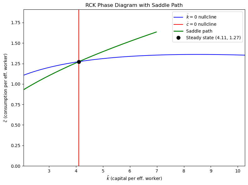
# Phase diagram
fig, ax = plt.subplots(figsize=(8,6))
k_grid = np.linspace(0.5*kstar, 2.5*kstar, 200)
c_nullcline = k_grid**alpha - mu0*k_grid    # dk/dt = 0 nullcline
ax.plot(k_grid, c_nullcline, 'b-', label=r'$\dot{k}=0$ nullcline')
ax.axvline(kstar, color='r', linestyle='-', label=r'$\dot{c}=0$ nullcline')
ax.plot(k_path, c_path, 'g-', linewidth=2, label='Saddle path')
# Mirror: perturb to the left
state0_left = [kstar - eps*v_stable[0], cstar - eps*v_stable[1]]
sol_left = solve_ivp(rck_backward, [0, 60], state0_left, max_step=0.01)
ax.plot(sol_left.y[0], sol_left.y[1], 'g-', linewidth=2)
ax.plot(kstar, cstar, 'ko', markersize=8, label=f'Steady state ({kstar:.2f}, {cstar:.2f})')
ax.set_xlabel(r'$\tilde{k}$ (capital per eff. worker)')
ax.set_ylabel(r'$\tilde{c}$ (consumption per eff. worker)')
ax.set_title('RCK Phase Diagram with Saddle Path')
ax.legend(); ax.set_xlim(0.5*kstar, 2.5*kstar); ax.set_ylim(0, 1.5*cstar)
plt.tight_layout(); plt.show()

Steady state: k* = 4.1059, c* = 1.2728
Eigenvalues: [ 0.14356784 -0.09356784]

Julia¶

using DifferentialEquations, LinearAlgebra

alpha, rho, sigma, delta = 1/3, 0.04, 2.0, 0.05
n, g = 0.01, 0.02; mu0 = n+g+delta

r_star = delta + rho + sigma*g
kstar = (alpha/r_star)^(1/(1-alpha))
cstar = kstar^alpha - mu0*kstar
println("k* = $(round(kstar,digits=4)), c* = $(round(cstar,digits=4))")

function rck!(du, u, p, t)
    k, c = u
    du[1] = k^alpha - c - mu0*k
    du[2] = (c/sigma)*(alpha*k^(alpha-1) - delta - rho - sigma*g)
end

# Jacobian at steady state
J = [alpha*kstar^(alpha-1)-mu0  -1;
     (cstar/sigma)*alpha*(alpha-1)*kstar^(alpha-2)  0.0]
λ, V = eigen(J)
println("Eigenvalues: $(round.(λ, digits=4))")

# Stable eigenvector
idx = argmin(real.(λ))
v = real(V[:,idx]); v = v/norm(v)

# Reverse shooting
rck_back!(du, u, p, t) = (rck!(du, u, p, t); du .= -du)
eps = 0.01
u0 = [kstar + eps*v[1], cstar + eps*v[2]]
prob = ODEProblem(rck_back!, u0, (0.0, 60.0))
sol = solve(prob, Tsit5(), saveat=0.1, reltol=1e-8)
println("Saddle path traced: $(length(sol.t)) points")

R¶

library(deSolve)

alpha <- 1/3; rho <- 0.04; sigma <- 2.0; delta <- 0.05
n <- 0.01; g <- 0.02; mu0 <- n+g+delta

r_star <- delta + rho + sigma*g
kstar <- (alpha/r_star)^(1/(1-alpha))
cstar <- kstar^alpha - mu0*kstar

rck_system <- function(t, state, pars) {
  k <- state[1]; c <- state[2]
  list(c(k^alpha - c - mu0*k,
         (c/sigma)*(alpha*k^(alpha-1) - delta - rho - sigma*g)))
}
rck_back <- function(t, state, pars) lapply(rck_system(t,state,pars), function(x) -x)

# Jacobian and stable eigenvector
J <- matrix(c(alpha*kstar^(alpha-1)-mu0, (cstar/sigma)*alpha*(alpha-1)*kstar^(alpha-2),
              -1, 0), 2, 2)
ev <- eigen(J)
idx <- which.min(Re(ev$values))
v <- Re(ev$vectors[,idx]); v <- v/sqrt(sum(v^2))

eps <- 0.01
state0 <- c(kstar + eps*v[1], cstar + eps*v[2])
sol <- ode(state0, seq(0,60,0.1), rck_back, parms=NULL, method="rk4")
cat(sprintf("Steady state: k*=%.4f, c*=%.4f\n", kstar, cstar))

11.8 Worked Example: Calibration to U.S. Data and Policy Experiments¶

Cross-reference: Principles Ch. 5.3 (policy experiments in the RCK model) [P:Ch.5.3]

Calibration: $\alpha = 1/3$ , $\delta = 0.05$ , $n = 0.01$ , $g = 0.02$ , $\rho = 0.04$ , $\sigma = 2$ . Then:

$\tilde{k}^* = (0.33/(0.05+0.04+0.02\times2))^{1/(2/3)} = (0.33/0.13)^{1.5} = (2.54)^{1.5} = 4.04$

$\tilde{c}^* = 4.04^{0.333} - 0.08\times4.04 = 1.593 - 0.323 = 1.270$

Implied saving rate: $s^* = 1 - \tilde{c}^*/\tilde{y}^* = 1 - 1.270/1.593 = 0.203$ — approximately 20%, consistent with U.S. data.

Policy experiment — Permanent increase in $g$ : A rise in technology growth from $g = 0.02$ to $g = 0.025$ :

New $r^{new} = \delta + \rho + \sigma g^{new} = 0.05 + 0.04 + 2\times0.025 = 0.14$ (up from 0.13).

New $\tilde{k}^{new} = (0.33/0.14)^{1.5} = (2.36)^{1.5} = 3.62$ (falls — faster technology means less capital needed per effective worker).

New $\tilde{c}^{new} = 3.62^{0.333} - 0.09\times3.62 = 1.535 - 0.326 = 1.209$ (falls in effective-worker units but rises in per-capita terms since $g$ is higher).

The transition path: On impact, the rise in $g$ reduces $\tilde{k}^*$ and $\tilde{c}^*$ . The economy must transition from the old to the new steady state along a new saddle path. On impact, $\tilde{k}$ cannot jump (it is a state variable), but $\tilde{c}$ can: it jumps to the new saddle path at the current $\tilde{k}$ , then evolves along the new saddle path to the new steady state.

11.9 Programming Exercises¶

Exercise 11.1 (APL — Euler Equation Verification)¶

Starting from the APL steady state computation, implement a discrete-time approximation to the Euler equation: $c_{t+1}/c_t = [\beta(1+r_t)]^{1/\sigma}$ with $r_t = f'(k_t) - \delta$ . Simulate a discrete-time RCK model on the Solow steady-state capital path and verify that the Euler equation holds along the transition path.

Exercise 11.2 (Python — Phase Diagram with Multiple Trajectories)¶

Plot the full RCK phase diagram: (a) nullclines; (b) saddle path (both branches); (c) four “wrong” trajectories (starting slightly off the saddle path) that either diverge to $k=0$ or $c<0$ ; (d) direction arrows in each of the four phase-plane quadrants. Label the saddle point and the Golden Rule capital stock.

Exercise 11.3 (Julia — Policy Experiment)¶

Simulate the RCK model response to a permanent increase in $\rho$ (a sudden increase in impatience from 0.04 to 0.06). (a) Compute the old and new steady states. (b) On impact, find $c_0^{new}$ using the reverse-shooting algorithm for the new saddle path evaluated at $k_0 = k^*_{old}$ . (c) Plot the transition path $(\tilde{k}(t), \tilde{c}(t))$ in the phase plane and as time series. (d) Characterize the transition: does consumption jump up or down on impact? Does capital increase or decrease toward its new steady state?

Exercise 11.4 (R — Convergence Rate)¶

For the linearized RCK system, the stable eigenvalue $\lambda_-$ gives the speed of convergence. Compute $\lambda_-$ as a function of $\sigma \in \{0.5, 1, 2, 5\}$ with other parameters fixed. Show that: (a) higher $\sigma$ (lower EIS) reduces $|\lambda_-|$ — convergence is slower with less intertemporal substitution; (b) compare to the Solow convergence rate $\lambda^{Solow} = (1-\alpha)\mu$ ; (c) the RCK model generally converges faster than the Solow model because forward-looking households adjust consumption more rapidly.

Exercise 11.5 — Stochastic Euler Equation ( $\star$ )¶

In the discrete-time version of the RCK model with i.i.d. productivity shocks $A_t$ , the Euler equation is $u'(c_t) = \beta\mathbb{E}_t[(1+r_{t+1})u'(c_{t+1})]$ . (a) With CRRA utility, show this can be written $c_t^{-\sigma} = \beta\mathbb{E}_t[(1+r_{t+1})c_{t+1}^{-\sigma}]$ . (b) Log-linearize around the steady state to get $\hat{c}_t = \mathbb{E}_t[\hat{c}_{t+1}] - (1/\sigma)(r_{t+1} - r^*)$ . (c) Show this is the NK IS curve up to the sign convention and the distinction between the interest rate and the marginal product of capital.

Exercise 11.6 — Decentralization ( $\star\star$ )¶

The RCK model can be solved either as a social planner’s problem (as above) or as a competitive equilibrium where households rent capital to firms. (a) Set up the household’s problem of maximizing lifetime utility subject to the budget constraint $\dot{a} = ra + w - c$ (where $a$ is wealth, $r$ is the rental rate, $w$ is the wage). (b) Write the Hamiltonian and derive the household Euler equation. (c) Show that the competitive equilibrium and the planner’s solution coincide when markets are complete (the First Welfare Theorem). (d) Identify the conditions under which the competitive equilibrium is also saddle-path stable.

11.10 Chapter Summary¶

Key results:

The Ramsey–Cass–Koopmans problem is an infinite-horizon optimal control problem: maximize lifetime utility $\int_0^\infty e^{-\rho t}u(\tilde{c})\,dt$ subject to $\dot{\tilde{k}} = f(\tilde{k}) - \tilde{c} - \mu_0\tilde{k}$ .
The current-value Hamiltonian $\mathcal{H} = u(\tilde{c}) + \mu[f(\tilde{k}) - \tilde{c} - \mu_0\tilde{k}]$ generates three necessary conditions via Pontryagin’s maximum principle: the FOC ( $\mu = u'(\tilde{c})$ ), the costate equation ( $\dot\mu = \rho\mu - \mu f'(\tilde{k}) + \mu\mu_0$ ), and the TVC.
Combining FOC and costate equation yields the Ramsey–Euler equation: $\dot{\tilde{c}}/\tilde{c} = [f'(\tilde{k}) - \delta - \rho - \sigma g]/\sigma$ — the continuous-time analogue of the discrete Euler equation.
The phase plane has one $\dot{\tilde{k}} = 0$ hump-shaped nullcline and one vertical $\dot{\tilde{c}} = 0$ nullcline; their intersection is the saddle-point steady state with $f'(\tilde{k}^*) = \delta + \rho + \sigma g$ .
The steady state is a saddle point because $\det(J) = \tilde{c}^*f''(\tilde{k}^*)/\sigma < 0$ , ensuring opposite-sign eigenvalues.
The reverse-shooting algorithm computes the saddle path numerically by perturbing slightly from the steady state along the stable eigenvector and integrating backward in time.
The TVC $\lim_{t\to\infty}e^{-\rho t}\mu\tilde{k} = 0$ selects the unique optimal trajectory (the saddle path) by ruling out Ponzi accumulation and unsustainable debt paths.

Connections forward: Chapter 13 applies the same Hamiltonian framework to the firm’s investment problem, deriving Tobin’s $q$ as the costate variable. Chapter 17 discretizes the RCK model into an RBC framework and solves it via value function iteration. Chapter 28 shows that the saddle-path condition of the RCK model is the prototype for the Blanchard–Kahn stability conditions of DSGE models.

Next: Chapter 12 — The Continuous-Time Overlapping Generations Model