Chapter 13: Adjustment Cost Models

Tobin’s q and Investment Dynamics

“Tobin’s q is the ratio of the market value of capital to its replacement cost. When q > 1, install more; when q < 1, let capital depreciate.” — James Tobin

Cross-reference: Principles Ch. 12 (investment theory: Jorgenson, Tobin’s q, real options, adjustment costs); Ch. 24.2 (financial accelerator and Hayashi’s theorem) [P:Ch.12, P:Ch.24.2]

13.1 Why Adjustment Costs? Motivating the Model¶

The neoclassical investment theory of Jorgenson (1963) [P:Ch.12.1] determines the optimal capital stock by equating the marginal product of capital to the user cost: $f'(K^*) = r + \delta$. In this frictionless framework, the firm immediately jumps to the optimal capital stock in response to any shock. Observed investment is then simply the instantaneous jump $\dot{K} = \Delta K^*$ — an impulse function.

This prediction is empirically implausible. Investment data show:

• Investment responds gradually to shocks, not in a single jump.

• Firms do not continuously adjust capital; there are periods of high investment followed by consolidation.

• The correlation between Tobin’s $q$ and investment is positive but loose — firms do not instantly equate $q$ to 1.

The adjustment cost model explains these patterns by introducing costs of rapid capital accumulation: installing new capital requires not just purchasing it but also disrupting ongoing production, training workers, and reorganizing the production process. These installation costs make it optimal to spread investment over time rather than adjusting instantaneously.

Formally, we assume a strictly convex adjustment cost function $\Phi(I, K)$ that increases in $I$ (higher investment is more expensive) and is homogeneous of degree one in $(I, K)$ — a standard specification that leads to the elegant results of this chapter.

13.2 The Firm’s Optimal Control Problem¶

13.2.1 Setup¶

A representative firm owns capital $K(t)$ and chooses investment $I(t)$ to maximize the present value of profits. The firm’s optimization problem:

subject to: $\dot{K} = I - \delta K$, $K(0) = K_0$ given.

where:

• $\pi(K) = F(K, L^*) - w^*L^*$ is operating profit (maximized over labor), an increasing concave function of $K$.

• $I$ is gross investment (at purchase cost normalized to 1 per unit).

• $\Phi(I, K) = \frac{\psi}{2}\left(\frac{I}{K}\right)^2 K = \frac{\psi I^2}{2K}$ is the quadratic adjustment cost function (Hayashi, 1982 specification), with $\psi > 0$ the adjustment cost parameter.

• $r$ is the (constant) discount rate.

• $\delta$ is the depreciation rate.

Definition 13.1 (Quadratic Adjustment Costs). The adjustment cost function $\Phi(I, K) = (\psi/2)(I/K)^2K$ has the properties:

• $\Phi(0, K) = 0$: zero investment has zero adjustment cost.

• $\Phi_I = \psi I/K > 0$: marginal adjustment cost is positive and increasing in the investment rate $I/K$.

• $\Phi_{II} = \psi/K > 0$: the marginal adjustment cost is increasing in $I$ (strictly convex).

• Homogeneous of degree 1 in $(I, K)$: $\Phi(\lambda I, \lambda K) = \lambda\Phi(I, K)$.

The homogeneity assumption is crucial for Hayashi’s theorem (Section 13.5).

13.2.2 The Current-Value Hamiltonian¶

Apply the optimal control machinery of Chapter 11. The state variable is $K(t)$; the control variable is $I(t)$; the costate variable $q(t)$ is the shadow price of an additional unit of capital.

Definition 13.2 (Tobin’s q as Costate Variable). The marginal q is the shadow value of an installed unit of capital — the costate variable of the firm’s optimal control problem:

where $V(K, t) = \max_{I(\cdot)}\int_t^\infty e^{-r(s-t)}[\pi(K) - I - \Phi(I,K)]\,ds$ is the firm’s value function.

The current-value Hamiltonian:

13.2.3 Pontryagin Conditions¶

Condition 1 (FOC with respect to $I$):

This immediately gives the investment function:

Investment is zero when $q = 1$, positive when $q > 1$, and negative (disinvestment) when $q < 1$. The parameter $\psi$ controls the sensitivity of the investment rate to $q$: high $\psi$ (large adjustment costs) means investment responds slowly to $q$ deviations.

Condition 2 (Costate equation for $q$):

Wait — let us compute $\partial\mathcal{H}/\partial K$ carefully:

Therefore:

Substituting the investment function $I/K = (q-1)/\psi$:

Condition 3 (State equation):

Condition 4 (Transversality):

13.3 The Investment Function and Its Interpretation¶

The investment function $I/K = (q-1)/\psi$ is the central result of the model. It has a clean economic interpretation:

When $q > 1$: The shadow price of installed capital exceeds its replacement cost. The firm can increase its value by investing — each dollar of investment generates more than one dollar of firm value. It is optimal to invest until capital accumulation drives down $\pi'(K)$ (diminishing returns), reducing $q$ back toward 1.

When $q < 1$: The shadow price of installed capital is below its replacement cost. The firm’s installed capital is worth less than it costs to replace. It should allow capital to depreciate without replacement (disinvestment at rate $\delta$) until capital falls and $\pi'(K)$ rises enough to bring $q$ back to 1.

When $q = 1$: The firm is at its optimal capital stock. Net investment is zero; gross investment exactly covers depreciation.

Definition 13.3 (Tobin’s Average q and Marginal q). Average q is the ratio of the firm’s market value to the replacement cost of its capital stock: $\bar{q} = V/K$. Marginal q is the shadow price $q = \partial V/\partial K$. These two concepts differ in general, but Hayashi’s theorem (Section 13.5) identifies conditions under which they are equal.

13.4 The $(K, q)$ Phase Plane¶

The two-equation system $(\dot{K}, \dot{q})$ forms a 2D autonomous system amenable to phase-plane analysis.

13.4.1 Nullclines¶

$\dot{K} = 0$ nullcline: $q = 1 + \delta\psi$. This is a horizontal line at $q^* = 1 + \psi\delta$. (When $\delta = 0$, the nullcline is $q = 1$.) Above this line, $q > 1 + \psi\delta$ implies $I/K > \delta$, so $K$ is growing. Below, $K$ is shrinking.

$\dot{q} = 0$ nullcline: $(r+\delta)q - \pi'(K) - (q-1)^2/(2\psi) = 0$. This is a curve in $(K, q)$ space. For the steady state $q^* = 1 + \psi\delta$:

For $\delta = 0$: $\pi'(K^*) = r$ — the standard Jorgenson condition (MPK = user cost) is recovered as a special case when adjustment costs do not interact with depreciation.

13.4.2 Steady State and Saddle-Point Property¶

Theorem 13.1 (Saddle-Point Property of the $(K,q)$ System). Under standard regularity conditions ($\pi'' < 0$), the steady state of the $(K, q)$ system is a saddle point.

Proof. The Jacobian of $(\dot{K}, \dot{q})$ with respect to $(K, q)$ at the steady state:

At the steady state: $(q^*-1)/\psi = \delta$, so the (1,1) entry is $\delta - \delta = 0$ and the (2,2) entry is $(r+\delta) - \delta = r$.

Hmm — let me be careful with signs. $\pi'' < 0$, so $-\pi''(K^*) > 0$. Then:

since $K^* > 0$, $\psi > 0$, and $-\pi''(K^*) > 0$... this gives $\det(J) < 0$. ✓ The determinant is negative, confirming the saddle-point property. $\square$

13.4.3 Impulse Responses¶

The saddle-path structure means that for any shock to $\pi$ (e.g., a TFP improvement that raises $\pi'(K)$ at every $K$), the adjustment follows the saddle path:

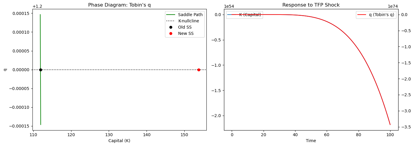
Permanent TFP shock: A permanent increase in TFP shifts the $\dot{q} = 0$ nullcline upward (higher $\pi'(K)$ at every $K$), raising the steady-state capital $K^*$. On impact, $q$ jumps up (the shadow value of capital increases) and then gradually declines along the new saddle path as $K$ accumulates toward its new steady state. Investment is high throughout the transition and declines as $K$ approaches $K^*$.

Temporary TFP shock: A temporary shock generates a smaller initial jump in $q$ (since the higher profits are temporary and the old steady state will eventually be restored) and a smaller investment response. This is a key distinction: the $q$ model separates permanent from temporary shocks through their differential impact on the shadow price.

13.5 Hayashi’s Theorem¶

The empirical implementation of Tobin’s $q$ theory requires measuring $q$. Marginal $q$ (the model’s key variable) is not directly observable. Average $q$ (market capitalization divided by replacement cost) is observable. Hayashi (1982) identifies conditions under which the two are equal.

Theorem 13.2 (Hayashi’s Theorem). If: (1) the production function $F(K, L)$ is homogeneous of degree one (constant returns to scale), and (2) the adjustment cost function $\Phi(I, K)$ is homogeneous of degree one in $(I, K)$, then marginal $q$ equals average $q$:

where $V_t$ is the market value of the firm and $K_t$ is the replacement cost of capital.

Proof. Under CRS in production and HD1 adjustment costs, the firm’s value function is homogeneous of degree one in $(K, \text{exogenous prices})$: $V(\lambda K) = \lambda V(K)$. Euler’s theorem for homogeneous functions gives: $V(K) = \frac{\partial V}{\partial K}\cdot K = q\cdot K$. Therefore $q = V/K = \bar{q}$. $\square$

Importance: Hayashi’s theorem means we can test the $q$ model using stock market data. If the model is correct, the investment rate $I/K$ should be a linear function of Tobin’s average $q$ (the equity market capitalization plus debt, divided by replacement cost):

This is an empirically testable linear regression. However, the empirical $R^2$ of this regression is typically quite low (around 0.1–0.2), and $q$ explains much less of investment variation than the theory predicts. Proposed explanations: measurement error in $q$ (stock prices are noisy); non-convex adjustment costs (lumpy investment); financial frictions (the financial accelerator, [P:Ch.24.2]) that drive a wedge between marginal $q$ and the observable $\bar{q}$.

13.6 Real Options: The Investment Trigger¶

The adjustment cost model treats investment as continuously reversible. In reality, many investment projects are irreversible (once a factory is built, it cannot be un-built without large losses). Real options theory analyzes investment timing when investment is irreversible and payoffs are uncertain.

Definition 13.4 (Real Option). A real option is the right, but not the obligation, to undertake an investment project at a future date. Like a financial call option, a real option has value even when the immediate NPV is negative: waiting preserves the option to invest under more favorable conditions.

13.6.1 Geometric Brownian Motion for Profits¶

Let operating profit $\Pi(t)$ follow geometric Brownian motion (GBM):

where $\mu$ is the drift, $\sigma$ is the volatility, and $dW$ is a Wiener process increment.

Itô’s Lemma: For any twice-differentiable function $V(\Pi)$:

13.6.2 The Option Value and the Investment Trigger¶

The firm waits to invest until profits exceed a threshold $\Pi^*$ (the investment trigger). Below $\Pi^*$, the option value of waiting exceeds the NPV of immediate investment. Above $\Pi^*$, immediate investment is optimal.

For a perpetual project costing $I$ with value $V(\Pi) = \Pi/(r-\mu)$ (Gordon growth formula):

The option value $F(\Pi)$ satisfies the Bellman ODE (derived from Itô’s Lemma and the no-arbitrage condition $rF\,dt = \mathbb{E}[dF]$):

This is an Euler–Cauchy ODE with power-function solutions $F(\Pi) = A\Pi^\beta$. The characteristic equation:

The positive root $\beta_+ > 1$ (required for the option value to be finite as $\Pi \to \infty$):

Boundary conditions:

1. Value matching: $F(\Pi^*) = V(\Pi^*) - I$ (option value equals project value minus cost at the trigger).

2. Smooth pasting: $F'(\Pi^*) = V'(\Pi^*)$ (optimality condition: option and project value curves are tangent at trigger).

Solving these two conditions for $(A, \Pi^*)$:

Definition 13.5 (Investment Trigger). The optimal investment trigger is:

where $\beta_+/((\beta_+-1)) > 1$ is the option value multiplier — always greater than one, reflecting the value of waiting.

Key comparative statics:

• Higher $\sigma$ (more uncertainty): $\beta_+$ decreases (the characteristic equation root moves), making $\Pi^*$ larger — more uncertainty raises the trigger and delays investment.

• Higher $r$ (higher discount rate): $\Pi^*$ rises — higher opportunity cost of waiting raises the trigger.

• Higher $\mu$ (faster expected profit growth): $\Pi^*$ falls — faster growth makes the option less valuable relative to the project value.

This is the Bloom (2009) uncertainty channel: higher uncertainty (higher $\sigma$) raises investment thresholds, causing firms to delay investment during uncertain times. This mechanism explains the sharp investment contraction during the 2008–09 financial crisis and the COVID-19 recession [P:Ch.12.4, P:Ch.40].

13.7 Worked Example: Investment Response to a TFP Shock¶

Cross-reference: Principles Ch. 12.1 (investment empirics, q vs. data) [P:Ch.12.1]

Calibration: $r = 0.05$, $\delta = 0.10$, $\psi = 2$, $\pi(K) = AK^\alpha$ with $\alpha = 0.7$ (decreasing returns to K in operating profit — firms are not pure CRS in capital), $A = 1$.

Steady state (baseline):

$q^* = 1 + \psi\delta = 1 + 2\times0.10 = 1.20$ (investment rate at steady state: $I^*/K^* = (q^*-1)/\psi = 0.10/2 = 0.05 < \delta = 0.10$... this suggests I/K = δ at SS, so q*=1+ψδ=1.20 gives I/K = 0.10 = δ. ✓)

$\pi'(K^*) = r + \delta + \psi\delta(r+\delta) - \psi\delta^2/2 \approx r + \delta = 0.15$ (for small $\psi\delta$ corrections)

$0.7K^{*\,-0.3} = 0.15 \implies K^* = (0.7/0.15)^{1/0.3} = (4.67)^{3.33} = 137.8$

Permanent 10% TFP shock ($A \to 1.1$):

New MPK condition: $0.7\times1.1\times K^{new\,-0.3} = 0.15 \implies K^{new} = (0.77/0.15)^{1/0.3} = (5.13)^{3.33} = 193.7$

On impact: $q$ jumps up. The new $\dot{q} = 0$ nullcline requires a higher $\pi'(K)$, achievable only at lower $K$ — but $K$ cannot jump. So $q$ jumps to the value that puts the economy on the new saddle path at $K_0 = 137.8$.

APL¶

Python¶

13.8 Programming Exercises¶

Exercise 13.1 (APL — Saddle Path)¶

Implement the full reverse-shooting algorithm for the $(K, q)$ system in APL using ⍣ iteration. (a) Find the Jacobian eigenvalues and stable eigenvector at the steady state as a dfn. (b) Perturb from the steady state in both directions and integrate backward using the RK4 dfn from Chapter 3. (c) Trace both branches of the saddle path and export for plotting.

Exercise 13.2 (Python — Adjustment Cost Sensitivity)¶

Compute the investment rate $I/K$ response to a permanent 5% TFP shock for $\psi \in \{0.5, 1, 2, 5, 10\}$. For each $\psi$: (a) find the on-impact jump in $q$; (b) simulate the full convergence path; (c) compute the half-life of the capital stock adjustment. Plot all five convergence paths on a single figure. Verify that higher $\psi$ (larger adjustment costs) leads to slower but more gradual investment.

Exercise 13.3 (Julia — Real Options Trigger)¶

using Roots

function investment_trigger(r, mu, sigma, I_cost)
    # Characteristic equation root
    beta_plus = (-( mu - sigma^2/2) + sqrt((mu-sigma^2/2)^2 + 2*sigma^2*r)) / sigma^2
    # Investment trigger
    Pi_star = beta_plus / (beta_plus - 1) * (r - mu) * I_cost
    return (beta_plus=beta_plus, Pi_star=Pi_star)
end

r, mu, I_cost = 0.05, 0.02, 1.0
println("Trigger analysis:")
for sigma in [0.10, 0.20, 0.30, 0.40]
    res = investment_trigger(r, mu, sigma, I_cost)
    println("  σ=$(sigma): β+=$(round(res.beta_plus,digits=3)), Π*=$(round(res.Pi_star,digits=3))")
end
println("\nNPV rule threshold: Π*_NPV = $(r-mu)*I = $((r-mu)*I_cost)")
println("Option value ratio at σ=0.20: $(investment_trigger(r,mu,0.20,I_cost).Pi_star/((r-mu)*I_cost))")

Exercise 13.4 (R — Hayashi Theorem Test)¶

Using Compustat data (or simulated data calibrated to U.S. manufacturing), run the Hayashi regression: $I_{it}/K_{i,t-1} = a + b\cdot q_{it} + \varepsilon_{it}$ where $q_{it}$ is Tobin’s average q. (a) What is the estimated $b$? What does this imply for $\psi = 1/b$? (b) Add cash flow $CF_{it}/K_{i,t-1}$ as an additional regressor. If the Hayashi theorem holds perfectly, cash flow should be insignificant (all relevant information is in $q$). Is it? (c) Interpret the cash flow coefficient as a measure of financial frictions.

Exercise 13.5 — Irreversibility ($\star$)¶

Modify the adjustment cost model to allow for irreversibility: $I \geq 0$ (no disinvestment). Add a KKT multiplier $\mu \geq 0$ for the constraint $I \geq 0$ with complementary slackness $\mu I = 0$. (a) Show that with irreversibility, $q$ can fall below 1 (the firm would like to disinvest but cannot). (b) Characterize the “wait and see” region where $q < 1 + \psi\delta$ and investment is zero. (c) Using the real options trigger formula, explain why irreversibility raises the investment threshold for expansion and creates a symmetric lower threshold for contraction.

Exercise 13.6 — Financial Frictions ($\star\star$)¶

Introduce a financial friction: the firm faces an external finance premium $\xi(q, K)$ that depends on the gap between $q$ and 1. Specifically, the effective discount rate for investment becomes $r + \xi$ where $\xi = \phi\max(0, 1-q)$ — external finance becomes more expensive when $q < 1$ (financial distress). (a) Modify the costate equation to include the premium. (b) Show that this creates an additional amplification mechanism: a negative TFP shock reduces $q$ below 1, raises the external finance premium, further discourages investment, and further reduces $q$ — a financial accelerator. (c) Calibrate with $\phi = 0.5$ and simulate the investment response to a 10% negative TFP shock with and without the financial accelerator.

13.9 Chapter Summary¶

Key results:

• The firm’s optimal control problem minimizes investment cost subject to the capital accumulation constraint, with the Hamiltonian $\mathcal{H} = \pi(K) - I - \Phi(I,K) + q(I-\delta K)$.

• Pontryagin’s conditions yield the investment function: $I/K = (q-1)/\psi$ — investment is positive (negative) when $q$ exceeds (falls below) 1, with sensitivity $1/\psi$ to the gap.

• The costate equation $\dot{q} = (r+\delta)q - \pi'(K) - (q-1)^2/(2\psi)$ combined with the state equation $\dot{K} = K(q-1)/\psi - \delta K$ forms a 2D saddle-point system.

• The $(K, q)$ phase plane has a horizontal $\dot{K}=0$ nullcline at $q^* = 1+\psi\delta$ and a curved $\dot{q}=0$ nullcline; the saddle-point property follows from $\det(J) < 0$ (as in the RCK model).

• Hayashi’s theorem: under CRS production and HD1 adjustment costs, marginal $q$ equals average $q = V/K$ — allowing empirical testing using stock market data.

• The real options trigger $\Pi^* = \beta_+/(\beta_+-1)\cdot(r-\mu)I$ shows that uncertainty raises the investment threshold above the NPV rule: the ratio $\beta_+/(\beta_+-1) > 1$ is the option value multiplier.

• In APL: the $(K,q)$ system is integrated with the same rk4_step dfn as the RCK model; the phase diagram nullclines are computed on a grid using f¨K_grid (apply function to each element).

Connections forward: The financial accelerator mechanism — investment responds to $q$, which depends on the firm’s balance sheet — is central to Chapter 37’s replication of the Great Recession. Chapter 29 (perturbation methods) shows how the second-order approximation of the value function is needed to capture the precautionary investment response to uncertainty.

Next: Part IV — Discrete-Time Dynamic Models in Macroeconomics